Lesson 3 of 6
Graphs, slopes and intercepts
A function gives one output for each permitted input. A graph places those input-output pairs together so we can inspect their relationship.
See where two pricing stories cross
QuickRide charges ₹50 plus ₹10 per kilometre. Steady charges ₹110 plus ₹7 per kilometre. A graph puts both rules on the same axes so you can see when the cheaper choice changes.
Which service is cheaper at 10 km? Could the answer reverse on a longer journey?
Need a quick refresher?
Each permitted x has one output. The intercept is meaningful mathematically even when x = 0 is outside a realistic application range.
Review Functions, domains and outputs →Graphs, slopes and the plan that costs less
1 · Observe
Two data plans, one decision
| Word | What it means |
|---|---|
| Slope | How much the output rises for each extra unit of input. |
| Intercept | The output when the input is zero. |
| Linear | Described by an intercept plus a slope times x: a straight line. |
| Intersection | The input where two rules give the same answer. |
| Fitting a line | Choosing the intercept and slope that best match noisy points. |
Plan A costs ₹199 a month plus ₹10 for each extra GB. Plan B costs ₹399 plus ₹4 per extra GB. Which should you choose? It depends on how much data you use, and the picture that answers it fastest is a graph.
2 · Express
Slope and intercept
A straight line is y = m x + c. The intercept c is the value at x = 0. The slope m is the change in y for one unit of x: rise over run.
3 · Visualize
Where they cross
| Extra GB | Plan A | Plan B |
|---|---|---|
| 0 | ₹199 | ₹399 |
| 10 | ₹299 | ₹439 |
| 20 | ₹399 | ₹479 |
| 30 | ₹499 | ₹519 |
| 40 | ₹599 | ₹559 |
Between 30 and 40 GB the order flips. Set the costs equal: 199 + 10x = 399 + 4x, so 6x = 200 and x = 33.33 GB, at a bill of about ₹532. Below 33 GB, plan A is cheaper. Above it, plan B wins.
- Plan A
- Plan B
See the numbers behind this picture
| Extra GB | Plan A | Plan B |
|---|---|---|
| 0 | 199 | 399 |
| 1 | 209 | 403 |
| 2 | 219 | 407 |
| 3 | 229 | 411 |
| 4 | 239 | 415 |
| 5 | 249 | 419 |
| 6 | 259 | 423 |
| 7 | 269 | 427 |
| 8 | 279 | 431 |
| 9 | 289 | 435 |
| 10 | 299 | 439 |
| 11 | 309 | 443 |
| 12 | 319 | 447 |
| 13 | 329 | 451 |
| 14 | 339 | 455 |
| 15 | 349 | 459 |
| 16 | 359 | 463 |
| 17 | 369 | 467 |
| 18 | 379 | 471 |
| 19 | 389 | 475 |
| 20 | 399 | 479 |
| 21 | 409 | 483 |
| 22 | 419 | 487 |
| 23 | 429 | 491 |
| 24 | 439 | 495 |
| 25 | 449 | 499 |
| 26 | 459 | 503 |
| 27 | 469 | 507 |
| 28 | 479 | 511 |
| 29 | 489 | 515 |
| 30 | 499 | 519 |
| 31 | 509 | 523 |
| 32 | 519 | 527 |
| 33 | 529 | 531 |
| 34 | 539 | 535 |
| 35 | 549 | 539 |
| 36 | 559 | 543 |
| 37 | 569 | 547 |
| 38 | 579 | 551 |
| 39 | 589 | 555 |
4 · Discover
Reading a slope back from data
Real bills have noise. Fitting a line to noisy points recovers the slope: with the plan A bills scattered by about ₹8, a fitted line gave slope 9.98 and intercept 201.1, close to the true 10 and 199. This is, in miniature, what linear regression does.
5 · Apply
Two worked examples
Example 1, a slope. Between 10 GB (₹299) and 30 GB (₹499): (499 − 299) ÷ (30 − 10) = 10 rupees per GB.
Example 2, a decision. A user who typically uses 25 extra GB pays ₹449 on A and ₹499 on B. A is cheaper by ₹50.
6 · Where it goes wrong
Three ways it goes wrong
7 · In Python
Plans and slopes in code
Here is how to implement it, step by step. The code below does exactly these steps, and every line is editable.
- Write each plan as intercept + slope × x.
- Set the two costs equal: 199 + 10x = 399 + 4x.
- Collect the x terms on one side: 6x = 200.
- Divide: x = 33.33 GB.
- Substitute back to get the bill at the crossing, about ₹532.
import numpy as np

# two data plans: (price per month, GB included beyond a base)
# plan A: 199 rupees base + 10 rupees per extra GB.  plan B: 399 rupees base + 4 rupees per extra GB
a = lambda gb: 199 + 10 * gb
b = lambda gb: 399 + 4 * gb
for gb in (0, 10, 20, 30, 40):
    print("extra GB", str(gb).rjust(2), "| A:", a(gb), "| B:", b(gb))

# slope between two points of a line
(x1, y1), (x2, y2) = (10, a(10)), (30, a(30))
print("slope of A =", (y2 - y1) / (x2 - x1), "rupees per GB | intercept (GB = 0):", a(0))

# where the lines cross: 199 + 10x = 399 + 4x
x_cross = (399 - 199) / (10 - 4)
print("lines cross at", round(x_cross, 2), "GB, bill", round(a(x_cross), 1))

# fit a line to noisy points and read the slope back
rng = np.random.default_rng(1)
gb = np.arange(0, 41, 4)
paid = a(gb) + rng.normal(0, 8, len(gb))
slope, intercept = np.polyfit(gb, paid, 1)
print("fitted slope", round(slope, 2), "intercept", round(intercept, 1))
extra GB 0 | A: 199 | B: 399
extra GB 10 | A: 299 | B: 439
extra GB 20 | A: 399 | B: 479
extra GB 30 | A: 499 | B: 519
extra GB 40 | A: 599 | B: 559
slope of A = 10.0 rupees per GB | intercept (GB = 0): 199
lines cross at 33.33 GB, bill 532.3
fitted slope 9.98 intercept 201.1Edit and run this code in your browser
Live Python
Two plans, a crossing point, and a fitted slope
Runs in your browser on your device. Nothing you type is sent anywhere, and nothing here changes your saved progress.
Press Ctrl+Enter (⌘+Enter on Mac) to run. Tab moves focus to the next control, as usual; use spaces to indent.
Predict, then explore
Before changing anything: For y = 2x + 3, imagine increasing only the fixed fee by 2. Will the line get steeper, or move upward without changing its slope?
Keep coefficient a = 2 and increase b from 3 to 5. Compare outputs at more than one input, then restore b and change a. The table gives precise values; the plotted line shows the pattern.
Playground
Read a line: where it starts and how fast it climbs
Every straight rule is y = a·x + b. The intercept b is the starting fee (where the line meets the price axis). The slope a is the price of one more kilometre. Change them one at a time.
- Rule
- y = 2x + 3
- Starts at (x = 0)
- 3
- Crosses y = 0 at
- x = -1.5
One step right (1 km more) moves the line up by 2. That is the slope: change in output ÷ change in input.
The general function explorer
Function Explorer
f(x) = 2x + 3. At x = 2, output = 7.
See the exact values behind the graph
| Input x | Selected output |
|---|---|
| -4 | -5 |
| -3 | -3 |
| -2 | -1 |
| -1 | 1 |
| 0 | 3 |
| 0.5 | 4 |
| 1 | 5 |
| 2 | 7 |
| 3 | 9 |
| 4 | 11 |
In your own words: what changed, and why did the output change with it?
Now you drive
Recover a line from two points
Given two readings, can you rebuild the rule? You will compute the slope, the intercept, and then run the line backward to find an input.
| Maths | Python | In plain words |
|---|---|---|
| a = Δy ÷ Δx | (q[1] - p[1]) / (q[0] - p[0]) | Rise over run. |
| b = y₁ − a·x₁ | p[1] - a * p[0] | Walk back to x = 0. |
| x = (y − b) ÷ a | (y - b) / a | Undo the line. |
Live Python
slope(), intercept(), x_for()
Runs in your browser on your device. Nothing you type is sent anywhere, and nothing here changes your saved progress.
Press Ctrl+Enter (⌘+Enter on Mac) to run. Tab moves focus to the next control, as usual; use spaces to indent.
Stuck? Show a worked solution (try first!)
# Two readings from the same line: (1, 5) and (3, 9)
p, q = (1.0, 5.0), (3.0, 9.0)

def slope(p, q):
    return (q[1] - p[1]) / (q[0] - p[0])

def intercept(p, a):
    return p[1] - a * p[0]

def x_for(y, a, b):
    return (y - b) / a

a = slope(p, q)
b = intercept(p, a)
print(f"y = {a}x + {b}")
print("price 11 happens at x =", x_for(11, a, b))
Experiment, then explain
Finish the TODOs, then try the quick experiments. Think about each question before opening its answer.
What goes wrong if both points have the same x?
Δx is 0, so you divide by zero. A vertical line has no single output for that input, so it is not a function of x.
The line is y = 2x + 3, the same rule as the fare machine, and a bill of 11 happens at x = 4.
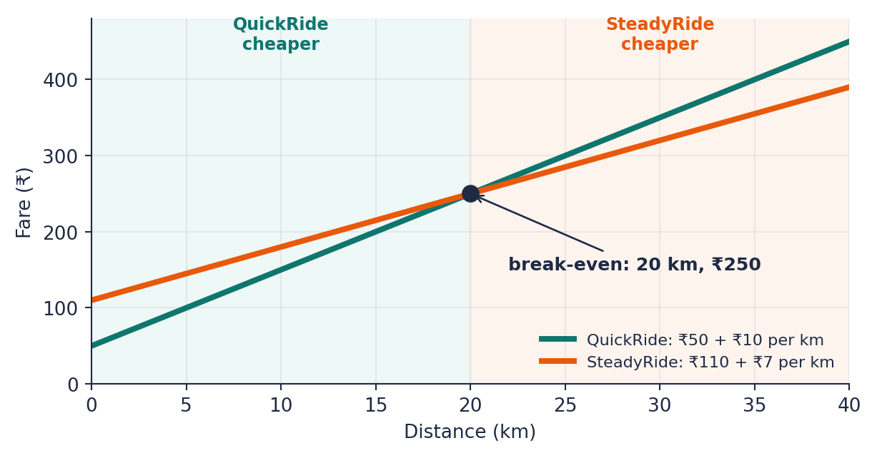
| Distance km | QuickRide ₹ | Steady ₹ |
|---|---|---|
| 0 | 50 | 110 |
| 10 | 150 | 180 |
| 20 | 250 | 250 |
| 30 | 350 | 320 |
The intercept is the starting charge. The slope is the added cost per kilometre. Setting 50 + 10d = 110 + 7d gives d = 20: the crossing represents equal prices, not equal slopes.
Relate the playground’s rule to this reading
A coordinate (x,y) pairs an input on the horizontal axis with an output on the vertical axis. For y = ax + b, b is the output at x = 0; a is the change in output divided by a nonzero change in input.
The points (1,5) and (3,9) have slope (9−5)/(3−1) = 2 rupees/km. Their line is y = 2x + 3. Raising b by 2 raises every output by 2. Raising a changes each output by the coefficient increase times x, so the effect depends on the input.
A positive slope rises, a negative one falls and zero is constant. A line shows a constant rate; a curved graph can show a changing rate. A visual angle depends on axis scaling, so use quantities and units to compare slopes.
Δ means change: slope = Δy/Δx. In ML, ŷ = wx + b uses a hat for an estimate and w for a coefficient. The same algebra does not establish a real-world causal effect.
A line is one family of relationships. Quadratics show changing rates and turning points, exponentials repeated proportional change, and logarithms the inverse growth question.
Explore other shapes and choose a useful chart
A graph lets you see a relationship.
An equation holds many possible input-output pairs in one compact rule. Plot those pairs and you can see a trend, a turning point or a surprising change. Read the axes, units and scale first; use the calculation or data table for precise values.
Schematic shape · axes not calibrated
Line: a constant amount per extra unit
y = 2x + 3 describes a fixed fee plus a price per kilometre.
Use a line to see rate and starting value. A steeper plotted angle alone is unreliable when axes use different scales.
Schematic shape · axes not calibrated
Quadratic: the change itself changes
y = x² describes the area of a square as its side changes.
Equal changes in side length do not add equal areas. A U-shaped squared-error curve can also help us see where a model's loss is smallest.
Schematic shape · axes not calibrated
Exponential: equal steps, equal factors
y = 2ˣ doubles whenever x increases by one.
Use it for repeated proportional growth. The same kind of curve can describe decay when the base lies between zero and one.
Schematic shape · axes not calibrated
Logarithm: ask the growth question backward
y = log₂(x) asks how many doublings take 1 to x.
Use logarithms to compare multiplicative scales and undo exponentials. Real logarithms require positive inputs.
What if you have observations rather than an equation?
A scatterplot shows paired measurements, such as house area and recorded price; a fitted line is a separate model of those points. A line chart often shows change over ordered time. A bar chart compares categories; a histogram groups numerical values into intervals to show a distribution. Statistics develops these data views further.
Choose the picture to match the question: a relationship, a trend, a comparison or a distribution. A useful graph helps us notice a pattern; it does not establish a cause or prove what happens between sampled points.
Symbol and unit reference
(x,y)- Input-output coordinate
Δy/Δx- Output difference divided by nonzero input difference
a or w- Slope, output units per input unit
b, ŷ- Intercept and predicted output
Another worked example
The points (1,5) and (3,9) have slope (9−5)/(3−1) = 2 output units per input unit. Their line is y = 2x + 3. At x = 0 the output is 3; at x = 4 it is 11.
Connect the relationship to Python
distance_km = [0, 1, 2, 3]
bills = [2 * x + 3 for x in distance_km]
points = list(zip(distance_km, bills))
# [(0, 3), (1, 5), (2, 7), (3, 9)]
The comprehension calculates one output per input. zip pairs corresponding values; plotting these pairs makes the rule visible. No chart is executed by this code block.
Why this matters for ML
Linear Regression learns w and b from data. This lesson explains what they do before introducing any training algorithm.
Try a different situation
A chart of house area and recorded prices shows a rising cloud of points. Is that the same thing as a known straight-line pricing equation?
Compare your reasoning
No. A scatterplot shows observations; a fitted line is a separate model of their relationship. Inspect spread, units and coverage. A rising pattern alone neither proves a straight-line rule everywhere nor establishes that changing area causes a particular price change.
Not scored or saved. Compare your reasoning, not just the answer.
Read a larger expression when you’re ready
The five-level Equation X-Ray connects these ideas to multiple inputs, curves, nested functions and indexed sums. Choose any level; advanced solving is not required.
Equation X-Ray · Read the structure, then explain it
Mathematics as a language
Start with a familiar rule and build toward a larger expression. Reading its pieces comes before solving advanced equations. You can explore any level.
One rule, many possibilities
A trip has a 3-rupee booking fee and costs 2 rupees per kilometre. How can one statement describe any permitted distance?
y = 2x + 3
Read the relationship before trying to solve it. This is an illustrative example, separate from the live experiment.
Choose a building block to inspect its role.
Read the operations: Multiply distance by its rate, then add the fee. If a bill is known, solving asks which distance makes both sides equal.
Build the expression from smaller operations
Choose a valid construction in the stated order. This exercise organizes dependencies; it does not claim every implementation must evaluate independent branches in this order.
What problem could this relationship represent?
A booking fee plus a distance charge is one possible interpretation; a fixed production setup cost plus a per-item charge has the same structure.
Context we still need: Symbols alone do not establish currency, physical meaning or whether negative distances are allowed.
Connect the operations to code
bill = 2 * distance_km + 3Read the code as a map of operations. It is not executed here; imports, shapes and numerical safeguards depend on the actual lesson.
Explain a changed situation
Your notes and reveals are temporary. This reading practice does not change lesson completion or saved assessment evidence.
Understanding checks
Use the worked reasoning above. Answers within 0.001 count as correct.
Carry this idea forward
Graphs reveal patterns; equations and data tables let us check quantities precisely.
Next, investigate a curve where equal input steps multiply the output instead of adding a fixed amount.
What the existing checks cover
- Calculate and interpret slope from two coordinates.
- Distinguish an intercept change from a slope change.
- Connect slope sign to increasing or decreasing outputs.
- Interpret a weighted-input prediction without assuming prior ML knowledge.
Build your lesson evidence
Try the experiment. 0 of 4 checks done.