Equation X-Ray · Read the structure, then explain it
Mathematics as a language
Read a prediction before adjusting it
Estimate a house price from area without confusing the estimate with its observed sale price.
ŷ = wx + b
Read the relationship before trying to solve it. This is an illustrative example, separate from the live experiment.
Choose a building block to inspect its role.
Read the operations: At x=2.5, multiply 42 × 2.5 = 105, then add 140 to get 245.
Build the expression from smaller operations
Choose a valid construction in the stated order. This exercise organizes dependencies; it does not claim every implementation must evaluate independent branches in this order.
What problem could this relationship represent?
A rate plus a baseline also describes many non-housing relationships.
Context we still need: A model relationship does not prove that changing area causes a price change in the world.
Connect the operations to code
prediction = coefficient * area + baselineRead the code as a map of operations. It is not executed here; imports, shapes and numerical safeguards depend on the actual lesson.
Explain a changed situation
Review the five-level equation-reading journey →
Your notes and reveals are temporary. This reading practice does not change lesson completion or saved assessment evidence.
Why draw a line through prices at all?
1 · Observe
You are asked to price a flat nobody has sold yet
| Word | What it means |
|---|---|
| Feature | A fact you know about each case, here the flat's area in sq m. |
| Target | The thing you want to predict, here the price in ₹ lakh. |
| Prediction (ŷ) | The model's guess for the target. Read 'y-hat'. |
| Baseline | The simplest sensible guess, here 'always the average price'. A model must beat it. |
| MAE | Mean absolute error: the average size of the misses, in the target's own unit (lakh). |
| Slope | How much the line rises for each extra unit of the feature. |
A buyer asks what a 75 sq m flat should cost. You have eight recent sales. The simplest answer ignores size: quote the average price. That is a fair opening move, and a weak one, because a 40 sq m flat and a 110 sq m flat do not sell for the same money.
Linear regression is the next simplest idea. Draw one straight line through the sales and read the price off it. Everything else in this module is about drawing that line well and knowing when to distrust it.
2 · Express
A prediction is a rule from inputs to a number
The input (feature) is area in sq m. The output (target) is price in ₹ lakh. A model is a rule that turns the first into an estimate of the second. The baseline rule says 'always the average'. The line rule says 'price depends on area'.
3 · Visualize
Eight flats, two rules
Areas 40 to 110 sq m with prices ₹30 to ₹84 lakh.
| Rule | Formula | Average miss (MAE) |
|---|---|---|
| Always the average | ₹53.6 lakh | ₹15.62 lakh |
| Fitted line | 0.806 × area − 6.82 | ₹3.98 lakh |
Using area cuts the typical miss from about ₹15.6 lakh to ₹4.0 lakh, a 75 percent reduction. For a 75 sq m flat, the line says 0.806 × 75 − 6.82 = ₹53.6 lakh, which happens to equal the average, because 75 is the average area and a fitted line passes through the point of averages.
- Sales
- Fitted line: average miss 4.0 lakh
- Average price: average miss 15.6 lakh
See the numbers behind this picture
| Area (sq m) | Sales | Fitted line: average miss 4.0 lakh | Average price: average miss 15.6 lakh |
|---|---|---|---|
| 35 | – | 21.387 | 53.625 |
| 40 | 30 | – | – |
| 50 | 34 | – | – |
| 60 | 36 | – | – |
| 70 | 52 | – | – |
| 80 | 55 | – | – |
| 90 | 58 | – | – |
| 100 | 80 | – | – |
| 110 | 84 | – | – |
| 115 | – | 85.863 | 53.625 |
4 · Discover
What 'fitted' means
Among all straight lines, we choose the one with the smallest average squared miss. The next lessons show how to write that line down, measure its misses, find it by repeated small steps, and extend it to many features.
5 · Apply
Two worked examples
Example 1, a small flat. 45 sq m: 0.806 × 45 − 6.82 = 29.5 lakh. The average rule would say 53.6, over 24 lakh too high.
Example 2, a big flat. 110 sq m: 0.806 × 110 − 6.82 = 81.8 lakh, against a recorded sale of 84. The line misses by 2.2 lakh, the average rule by 30.4 lakh.
6 · Where it goes wrong
Three ways it goes wrong
7 · In Python
The line against the average
Here is how to implement it, step by step. The code below does exactly these steps, and every line is editable.
- Put the eight sales into two lists: area and price.
- Make the baseline: guess the average price for every flat, and measure its average miss (15.62 lakh).
- Fit a straight line with np.polyfit(area, price, 1). It returns the slope and the starting height.
- Measure the line's average miss (3.98 lakh) and compare it with the baseline.
- Use the line on a flat nobody has sold: price = slope × area + height.
import numpy as np

area = np.array([40, 50, 60, 70, 80, 90, 100, 110], float)
price = np.array([30, 34, 36, 52, 55, 58, 80, 84], float)           # lakh rupees

guess_avg = np.full_like(price, price.mean())
w, b = np.polyfit(area, price, 1)
guess_line = w * area + b
mae = lambda p: np.abs(price - p).mean()
print("average price:", round(price.mean(), 1), "lakh | MAE of always guessing it:", round(mae(guess_avg), 2))
print("fitted line: price = %.3f x area + %.2f" % (w, b), "| MAE of the line:", round(mae(guess_line), 2))
print("a 75 sq m flat -> line says", round(w * 75 + b, 1), "lakh")
average price: 53.6 lakh | MAE of always guessing it: 15.62
fitted line: price = 0.806 x area + -6.82 | MAE of the line: 3.98
a 75 sq m flat -> line says 53.6 lakhEdit and run this code in your browser
Live Python
Fit a line to eight sales and compare with the average
Runs in your browser on your device. Nothing you type is sent anywhere, and nothing here changes your saved progress.
Press Ctrl+Enter (⌘+Enter on Mac) to run. Tab moves focus to the next control, as usual; use spaces to indent.
Want to implement it? Open the step-by-step playbook · How to choose a model
Learning objectives
Start with the decision, not the equation.
- Recognize a numerical prediction problem.
- Distinguish features from the target.
- Decide when a straight-line model is a useful baseline—and when it is not.
Problem and motivation
A housing analyst needs a useful first estimate.
Imagine a fictional housing team reviewing six homes. Before commissioning a detailed valuation, they want a consistent estimate from one known feature: floor area. Each row is an observation. Floor area is the feature we know; price is the numerical target we want to estimate.
Regression means predicting a number. Classification instead chooses a category. Neither is automatically “better”—they answer different questions.
Predict before reveal
If the observed relationship continues, which home should receive the larger price estimate?
Interactive exploration
Move one feature and observe the estimate.
This line summarizes a trend; it does not memorize every observed price.
- Input feature
- 2.5k ft²
- Model estimate
- ₹245 lakh
When to use it
A reasonable starting point
- The target is numerical.
- A roughly straight trend is plausible.
- You need an interpretable baseline.
- Residuals can be checked afterward.
Pause or choose another approach
- The desired output is a category.
- The relationship is strongly curved or discontinuous.
- Important variables are missing.
- Outliers or extrapolation dominate the decision.
Lesson summary
Connect the final pieces
Linear Regression predicts a numerical target from features by fitting a straight relationship. Predictions are estimates, so residuals are expected and must be evaluated. It is a useful, interpretable baseline—not a guarantee that the world is linear.
Complete the prediction, move the feature control, and answer both decision checks.Explore the book’s separate housing example
A useful prediction starts with a question
A buyer asks what an unlisted flat might cost. Past sales supply observed areas and recorded prices. A model supplies an estimate for a new area; it does not reveal a hidden true price.
The playground uses a separate dataset. Compare with the illustrated example ↓
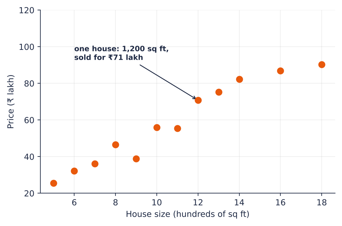
Source: Linear Regression · Book 8, PDF pages 4–5. Static source illustration; annotated scores belong to this example.
| Quantity | Role |
|---|---|
| Area | Known input |
| Recorded price | Observed target |
| Predicted price | Calculated estimate |
predicted price = intercept + slope × area
The feature is the supplied area; the target is the recorded sale price. Training chooses the slope and intercept using permitted past observations.
Return to the playground and explain how its inputs connect to this relationship. Unscored reading.