Linear Regression: How Gradient Descent Learns

Equation X-Ray · Read the structure, then explain it

Mathematics as a language

Read a prediction before adjusting it

Estimate a house price from area without confusing the estimate with its observed sale price.

ŷ = wx + b

Read the relationship before trying to solve it. This is an illustrative example, separate from the live experiment.

Choose a building block to inspect its role.

Read the operations: At x=2.5, multiply 42 × 2.5 = 105, then add 140 to get 245.

Build the expression from smaller operations

Choose a valid construction in the stated order. This exercise organizes dependencies; it does not claim every implementation must evaluate independent branches in this order.

What problem could this relationship represent?

A rate plus a baseline also describes many non-housing relationships.

Context we still need: A model relationship does not prove that changing area causes a price change in the world.

Connect the operations to code

prediction = coefficient * area + baseline

Read the code as a map of operations. It is not executed here; imports, shapes and numerical safeguards depend on the actual lesson.

Explain a changed situation

If w increases by 4 and x stays 2.5, how much does the prediction change? Would every input change by that amount?

Review the five-level equation-reading journey →

Your notes and reveals are temporary. This reading practice does not change lesson completion or saved assessment evidence.

The full story · about 14 minutes

Finding the line by walking downhill

1 · Observe

Guess, check, nudge

Words used in this lesson
Word	What it means
Loss	One number saying how wrong the model is right now. Here the mean squared error.
Gradient	The slope of the loss: it says which way, and how steeply, the loss changes if you nudge a weight.
Gradient descent	Repeatedly nudging the weights against the slope so the loss falls.
Learning rate (η)	The size of each step. Too small is slow; too big overshoots.
Standardise	Rescale a feature to average 0 and spread 1, so one learning rate suits every feature.

We could solve for the best line with algebra. Most models in this course cannot be solved that way, so we use a method that works everywhere: start with a guess, see which direction lowers the error, step that way, and repeat. This is gradient descent.

2 · Express

The update

For the mean squared error, the slope of the error with respect to each parameter is the average of (prediction − actual) times the input, and for the bias, the average of (prediction − actual). Move each parameter against its slope, scaled by the learning rate η.

w ← w − η · mean[(ŷ − y) · x]

b ← b − η · mean[ŷ − y]

Standardising x first (mean 0, spread 1) lets one learning rate work for both parameters.

3 · Visualize

Five learning rates

Same eight flats, area standardised, starting from w = 0 and b = 0. The best possible MSE is 21.0.

Mean squared error by learning rate
Learning rate η	After 10 steps	After 200 steps
0.01	2705.3	79.9
0.1	503.8	21.0
0.5	21.0	21.0
1.0	21.0	21.0
2.1	17905.3	diverged

A tiny rate is safe but slow: after 200 steps it has not arrived. Rates of 0.5 and 1.0 arrive in about ten steps. At 2.1 each step overshoots the valley by more than it gained, and the error explodes.

Loss against steps, for three learning rates

η = 0.01
η = 0.1
η = 0.5

See the numbers behind this picture

Loss against steps, for three learning rates
Step	η = 0.01	η = 0.1	η = 0.5
0	3,237.625	3,237.625	3,237.625
1	3,173.613	2,626.46	825.131
2	3,110.876	2,131.416	222.007
3	3,049.387	1,730.43	71.226
4	2,989.121	1,405.632	33.531
5	2,930.055	1,142.545	24.107
6	2,872.164	929.445	21.751
7	2,815.425	756.834	21.162
8	2,759.815	617.019	21.015
9	2,705.312	503.769	20.978
10	2,651.894	412.036	20.969
11	2,599.538	337.733	20.967
12	2,548.225	277.547	20.966
13	2,497.932	228.797	20.966
14	2,448.641	189.309	20.966
15	2,400.33	157.324	20.966
16	2,352.98	131.416	20.966
17	2,306.573	110.43	20.966
18	2,261.09	93.432	20.966
19	2,216.511	79.663	20.966
20	2,172.82	68.511	20.966
21	2,129.998	59.477	20.966
22	2,088.028	52.16	20.966
23	2,046.894	46.233	20.966
24	2,006.578	41.432	20.966
25	1,967.064	37.544	20.966
26	1,928.337	34.394	20.966
27	1,890.38	31.843	20.966
28	1,853.179	29.776	20.966
29	1,816.718	28.102	20.966
30	1,780.982	26.746	20.966
31	1,745.958	25.648	20.966
32	1,711.631	24.758	20.966
33	1,677.986	24.038	20.966
34	1,645.012	23.454	20.966
35	1,612.693	22.981	20.966
36	1,581.018	22.598	20.966
37	1,549.973	22.288	20.966
38	1,519.545	22.037	20.966
39	1,489.724	21.833	20.966

4 · Discover

It lands where the algebra does

With η = 0.5 the walk ends at 0.806 × area − 6.82, the same line as the exact solution, after converting from standardised back to raw units. Gradient descent is not a different model. It is a different way to find the same one.

5 · Apply

Two worked examples

Example 1, a step. At w = 0, b = 0 with standardised x, the average of (ŷ − y) is −53.6, the negative of the average price. With η = 0.5 the bias jumps from 0 to 26.8 in one step.

Example 2, a stop rule. Stop when the error barely changes, for example by less than 0.001 between steps, or after a fixed budget. Plot the error against the step number: it should fall smoothly.

Check yourself

The error rises every step. What is the most likely cause?

The learning rate is too small The learning rate is too large The data is perfect

6 · Where it goes wrong

Three ways it goes wrong

7 · In Python

Gradient descent in code

Here is how to implement it, step by step. The code below does exactly these steps, and every line is editable.

Standardise the area, so one learning rate works.
Start with w = 0 and b = 0, so the model predicts 0 for every flat.
Compute each flat's miss: prediction minus actual.
Update w by minus the learning rate times the average of (miss × input), and b by minus the learning rate times the average miss.
Repeat for many steps while watching the loss fall.

Five learning rates, and the line gradient descent finds

import numpy as np

area = np.array([40, 50, 60, 70, 80, 90, 100, 110], float)
price = np.array([30, 34, 36, 52, 55, 58, 80, 84], float)
w_exact, b_exact = np.polyfit(area, price, 1)

x = (area - area.mean()) / area.std()           # standardise so one learning rate suits both
def run(lr, steps=200):
    w = b = 0.0
    hist = []
    for s in range(steps):
        err = (w * x + b) - price
        w -= lr * (err * x).mean()
        b -= lr * err.mean()
        hist.append(float((err ** 2).mean()))
    return w, b, hist
for lr in [0.01, 0.1, 0.5, 1.0, 2.1]:
    w, b, h = run(lr)
    print("lr", str(lr).ljust(4), "| loss after 10 steps", round(h[9], 1), "| after 200 steps", "diverged" if h[-1] > 1e6 else round(h[-1], 1))
w, b, h = run(0.5)
slope = w / area.std()
intercept = b - w * area.mean() / area.std()
print("gradient descent line: %.3f x area + %.2f" % (slope, intercept), "| exact: %.3f x area + %.2f" % (w_exact, b_exact))

lr 0.01 | loss after 10 steps 2705.3 | after 200 steps 79.9
lr 0.1  | loss after 10 steps 503.8 | after 200 steps 21.0
lr 0.5  | loss after 10 steps 21.0 | after 200 steps 21.0
lr 1.0  | loss after 10 steps 21.0 | after 200 steps 21.0
lr 2.1  | loss after 10 steps 17905.3 | after 200 steps diverged
gradient descent line: 0.806 x area + -6.82 | exact: 0.806 x area + -6.82

Edit and run this code in your browser

Live Python

Five learning rates, and the line gradient descent finds

Runs in your browser on your device. Nothing you type is sent anywhere, and nothing here changes your saved progress.

Python code (editable)

Press Ctrl+Enter (⌘+Enter on Mac) to run. Tab moves focus to the next control, as usual; use spaces to indent.

Want to implement it? Open the step-by-step playbook · How to choose a model

The big idea

Lost on a foggy hill

Imagine standing on a hillside at night, in thick fog. You cannot see the valley, but you can feel the ground tilt under your feet. So you do the only sensible thing: take a small step in the direction that goes downhill, feel the slope again, and repeat.

That is how a machine learns. The hill is the loss: for every possible setting of the line (a slope w and a baseline b), the height tells us how wrong the predictions are. The valley floor is the best line. The slope under your feet is the gradient, which calculus gives us exactly. No machine ever sees the whole hill, only the slope where it stands, and that is enough.

Predict before you read on

Which way is downhill?

Our line starts at w = 10, b = 100. At that spot the slope of the hill is −892.5 in the w direction. It is negative: loss goes down as w goes up. Which step should we take?

Increase w a little Decrease w a little I can't tell yet

Problem and motivation

A training run produces poor estimates. We need a repeatable way to adjust both parameters and diagnose whether learning is working.

Build the intuition

Start with one house: a prediction below its recorded price has a negative residual. An update changes the rule, not the home. Inspect one update in the housing lab before reading the derivative formulas below. Loss is a height on a landscape of parameter settings. A derivative measures the local slope in one parameter direction. The gradient collects these slopes; descent takes a small step downhill.

What you will learn

Connect derivatives to a training decision

Explain why descent moves opposite the gradient.
Trace a simultaneous parameter update numerically.
Diagnose learning-rate instability from a sequence of losses.
Distinguish optimization evidence from generalization.

Need a quick concept reminder?

Concept bridge

Recall the concepts you will use

Connect these familiar ideas to this lesson before using the notation. Follow a review link if the prerequisite feels unfamiliar.

Mean Squared Error (MSE)(1/m)Σr²: The average squared residual.Squaring prevents cancellation and gives large misses extra influence.
Gradient∇L: A collection of derivatives describing how loss changes as parameters change.Its sign and size tell us which local parameter movement changes error most strongly.Review derivatives and gradients →
Learning rateα: The step-size multiplier used in a parameter update.Too small can learn slowly; too large can overshoot or diverge.
Parameterw, b: A model value learned or adjusted during training.Weight w controls how strongly a feature changes the prediction; bias b sets the baseline.Review weighted sums →

Guided experiment

Predict the update direction before pressing Step. Inspect iteration 0 and iteration 1 in the table. Compare the small, moderate and excessive presets from the same initial state. Describe the loss evidence before labelling the run.

Change a lab parameter or inspect another training state or diagnostic scenario, then answer the checks.

Real-world question

How do repeated gradient updates move a prediction line toward the data?

Predict before experimenting

Which learning rate is most likely to overshoot on this dataset?

0.001 1.0

Iteration: 0
Weight: 10
Bias: 100
MSE: 20,163.8333
Weight gradient: -892.5
Status: running

Actual observation Predicted point Regression line

Loss by parameter state · select any point to inspect it

Training history from the mathematical runtime
Iteration	Weight	Bias	MSE	Weight gradient	Bias gradient	Status
0	10	100	20,163.8333	-892.5	-269	running
1	18.925	102.69	12,413.8473	-699.1719	-212.1525	running
2	25.9167	104.8115	7,652.3527	-547.6394	-167.5905	running
3	31.3931	106.4874	4,726.8912	-428.867	-132.6582	running
4	35.6818	107.814	2,929.4299	-335.7725	-105.2737	running
5	39.0395	108.8667	1,824.9762	-262.8046	-83.8053	running
6	41.6676	109.7048	1,146.2848	-205.6124	-66.9742	running
7	43.7237	110.3745	729.1689	-160.7854	-53.7777	running
8	45.3315	110.9123	472.7575	-125.6504	-43.4302	running
9	46.588	111.3466	315.0784	-98.1122	-35.3157	running
10	47.5692	111.6998	218.0584	-76.5284	-28.9516	running
11	48.3344	111.9893	158.306	-59.6119	-23.9595	running
12	48.9306	112.2289	121.4507	-46.3535	-20.0427	running
13	49.3941	112.4293	98.6635	-35.9626	-16.9687	running
14	49.7537	112.599	84.5201	-27.8191	-14.5555	running
15	50.0319	112.7446	75.6881	-21.4372	-12.6602	running
16	50.2463	112.8712	70.1201	-16.4362	-11.1708	running
17	50.4106	112.9829	66.5582	-12.5173	-9.9995	running
18	50.5358	113.0829	64.2297	-9.4468	-9.0777	running
19	50.6303	113.1736	62.6598	-7.0412	-8.3514	running
20	50.7007	113.2572	61.5569	-5.1568	-7.7783	completed

Explain the observation

Describe only what the trace demonstrates.

Loss decreased across the inspected states, which shows optimization progress. This short trace alone does not establish convergence or generalization.

Each point is a complete parameter state. Iteration 0 is before any update; iteration 0 is after 0 successful updates.

Apply it

Compare small, moderate, and excessive rates.

Run each preset from iteration 0. Find one smooth decrease and one sequence that increases, oscillates, or terminates. Use the loss chart and runtime status as evidence.

Mathematical reasoning

L = (1/m) Σ rᵢ² is mean squared error over m observations, with rᵢ = ŷᵢ − yᵢ. Squaring stops positive and negative errors cancelling, and emphasizes large misses. A loss function turns many prediction errors into one optimization target.

For one feature, ∂L/∂w = (2/m) Σ rᵢxᵢ and ∂L/∂b = (2/m) Σ rᵢ. The chain rule supplies the feature factor for the weight derivative; the derivative of a prediction with respect to bias is 1. Gradients describe sensitivity of the entire dataset loss, not one selected residual.

A positive derivative means increasing that parameter locally increases loss. The gradient points in the direction of steepest local increase under the usual Euclidean distance. Hence w_new = w − α∂L/∂w and b_new = b − α∂L/∂b. Both derivatives must be computed from the same pre-update state. A negative derivative makes the subtraction increase the parameter.

Separate small-number worked example (not the housing lab settings): for inputs [1,2], targets [3,5], w = 1, b = 0: predictions [1,2], residuals [−2,−3], weight gradient −8, bias gradient −5. With learning rate α = 0.1 the next state is w = 1.8, b = 0.5. The runtime computes the exercise answer from this training trace.

Learning rate multiplies the update, not the gradient itself. A small rate can make slow progress; a large rate can overshoot, oscillate, increase loss, or eventually produce numerical divergence. A single increase is not proof of divergence. For this convex squared-error linear model an appropriate step can approach a minimum, but a short decreasing trace does not prove convergence or useful unseen predictions. Compare changes over many iterations, finite gradients and held-out error. Differently scaled features can make one shared rate awkward.

Mathematical symbol key

L, m, Σ, i: Dataset loss, observation count, sum, and observation index
rᵢ, xᵢ, yᵢ, ŷᵢ: Residual, input, observed and predicted target for row i
∂, ∇L: Partial derivative operator and vector of loss derivatives
w, b, α: Weight, bias and positive learning rate
new: Parameter after one simultaneous update

Real-world application

An energy-demand training job shows exploding loss after a rate change. Reduce the rate, inspect feature scales fitted on training data, and check finite updates. Select model settings using validation data; reserve test data for final evaluation.

Guided exercises and misconception checks

Explain the consequence of a change or choose a defensible action. Each check can be retried after the worked feedback. Successful checks remain recorded when you return.

1. The weight derivative is positive. Which small update locally moves downhill?Increase weight by adding the derivativeDecrease weight by subtracting a positive rate times the derivativeSet bias to zero

2. For the worked two-row example with w = 1, dw = −8 and α = 0.1, what is the next weight?Numerical answer

3. Loss goes 100, 40, 60, 150 after increasing the rate. What should you do first?Declare mastery because loss once decreasedTry a smaller rate from the same starting state and compare the full traceAdd the gradient to guarantee convergence

4. Training MSE falls steadily. What can you conclude?The optimizer reduced observed training loss; held-out performance still needs checkingThe model generalizes perfectlyAll learning rates converge

Now you drive

Code gradient descent yourself

The lab above ran the algorithm for you. Now write its heart: three lines of Python. The equations from this lesson become code almost word for word:

Maths and Python, side by side
Maths	Python	In plain words
rᵢ = ŷᵢ − yᵢ	`r = predict(w, b, xi) - yi`	How wrong is row i? (prediction minus actual)
∂L/∂w = (2/m) Σ rᵢ xᵢ	`dw += 2 / m * r * xi`	The Σ is the loop; each row adds its share. Steeper where the input xᵢ is large.
∂L/∂b = (2/m) Σ rᵢ	`db += 2 / m * r`	Same, without xᵢ: the baseline multiplies 1.
w ← w − α ∂L/∂w	`w = w - lr * dw`	Step against the slope. α is lr, the size of the step.

Fill in TODO 1, TODO 2 and TODO 3, then press Check my code. Before you finish, the program already runs; with the TODOs empty, the line just never moves. Notice what the loss curve does.

Live Python

Gradient descent on the housing data

Runs in your browser on your device. Nothing you type is sent anywhere, and nothing here changes your saved progress.

Quick experiments:

Python code (editable)

# ── Settings you can change ────────────────────────────
lr = 0.01            # learning rate: how big each downhill step is
steps = 20           # how many steps to take
w0, b0 = 10.0, 100.0 # starting guess:  price = w × area + b

# ── The data: area (thousand ft²) → price (₹ lakh) ──
X = [1.0, 1.8, 2.5, 3.2, 4.0, 4.8]
y = [178, 213, 246, 278, 316, 349]
m = len(X)

def predict(w, b, x):
    return w * x + b

def loss(w, b):
    # mean squared error: the height of the hill at (w, b)
    return sum((predict(w, b, xi) - yi) ** 2 for xi, yi in zip(X, y)) / m

def gradients(w, b):
    dw, db = 0.0, 0.0
    for xi, yi in zip(X, y):
        r = predict(w, b, xi) - yi    # residual: prediction − actual
        dw += 0.0                     # TODO 1: this row's share of ∂L/∂w
        db += 0.0                     # TODO 2: this row's share of ∂L/∂b
    return dw, db

w, b = w0, b0
history = [loss(w, b)]                # loss before any step
for step in range(steps):
    dw, db = gradients(w, b)
    # TODO 3: step downhill. Update w and b using lr, dw and db.
    history.append(loss(w, b))

print(f"start:  w = {w0:.2f}   b = {b0:.2f}   loss = {history[0]:.1f}")
print(f"after {steps} steps:  w = {w:.2f}   b = {b:.2f}   loss = {history[-1]:.1f}")

Press Ctrl+Enter (⌘+Enter on Mac) to run. Tab moves focus to the next control, as usual; use spaces to indent.

Stuck? Show a worked solution (try first!)

# ── Settings you can change ────────────────────────────
lr = 0.01            # learning rate: how big each downhill step is
steps = 20           # how many steps to take
w0, b0 = 10.0, 100.0 # starting guess:  price = w × area + b

# ── The data: area (thousand ft²) → price (₹ lakh) ──
X = [1.0, 1.8, 2.5, 3.2, 4.0, 4.8]
y = [178, 213, 246, 278, 316, 349]
m = len(X)

def predict(w, b, x):
    return w * x + b

def loss(w, b):
    # mean squared error: the height of the hill at (w, b)
    return sum((predict(w, b, xi) - yi) ** 2 for xi, yi in zip(X, y)) / m

def gradients(w, b):
    dw, db = 0.0, 0.0
    for xi, yi in zip(X, y):
        r = predict(w, b, xi) - yi    # residual: prediction − actual
        dw += 2 / m * r * xi              # (2/m) · rᵢ · xᵢ
        db += 2 / m * r                   # (2/m) · rᵢ
    return dw, db

w, b = w0, b0
history = [loss(w, b)]                # loss before any step
for step in range(steps):
    dw, db = gradients(w, b)
    w = w - lr * dw                   # w ← w − α · ∂L/∂w
    b = b - lr * db                   # b ← b − α · ∂L/∂b
    history.append(loss(w, b))

print(f"start:  w = {w0:.2f}   b = {b0:.2f}   loss = {history[0]:.1f}")
print(f"after {steps} steps:  w = {w:.2f}   b = {b:.2f}   loss = {history[-1]:.1f}")

Experiment, then explain

Finish the three TODOs, then use the quick experiments (or edit lr and steps yourself). Think about each question before opening its answer.

With lr = 0.001 the loss barely moves. Is the code broken?

No. The same correct code takes tiny steps, so after 20 of them the loss has only fallen from 20,164 to about 8,451 and w is still near 25. Try steps = 500: small steps are safe, just slow.

At lr = 0.05 the loss drops from 20,164 to about 198 in one step. Why does lr = 0.1 blow up?

At 0.05 the first step already overshoots the valley floor (the slope flips from negative to positive), but each later step lands closer. At 0.1 every overshoot is bigger than the last, so the loss grows instead of shrinking: after 20 steps it is about 8 million. The step size has to be small enough for each correction to shrink the error.

Why is the slope for b (−269) smaller than for w (−892.5)?

Each row’s share of ∂L/∂w is multiplied by its area xᵢ (up to 4.8), but ∂L/∂b is multiplied by 1. A feature measured in larger numbers has a steeper slope, which is why the next lessons talk about scaling features.

Same numbers, two ways: at lr = 0.01, 20 steps, this code ends at w ≈ 50.70, b ≈ 113.26, loss ≈ 61.6, exactly the iteration-20 row of the guided lab above, which runs on the platform’s verified TypeScript maths runtime.

Build the evidence

0 of 4 checks complete. Experiment interaction still required.

Completion records these objectives locally; it does not award mastery. Independent mastery will require unfamiliar examples and critical-objective evidence in the later assessment.

Explore the book’s separate housing example

Move the settings toward smaller error

For observations (1,2), (2,3), (3,5), a least-squares line has slope 1.5 and intercept 1/3. A formula and an iterative search can solve the same objective under suitable conditions.

The playground uses a separate dataset. Compare with the illustrated example ↓

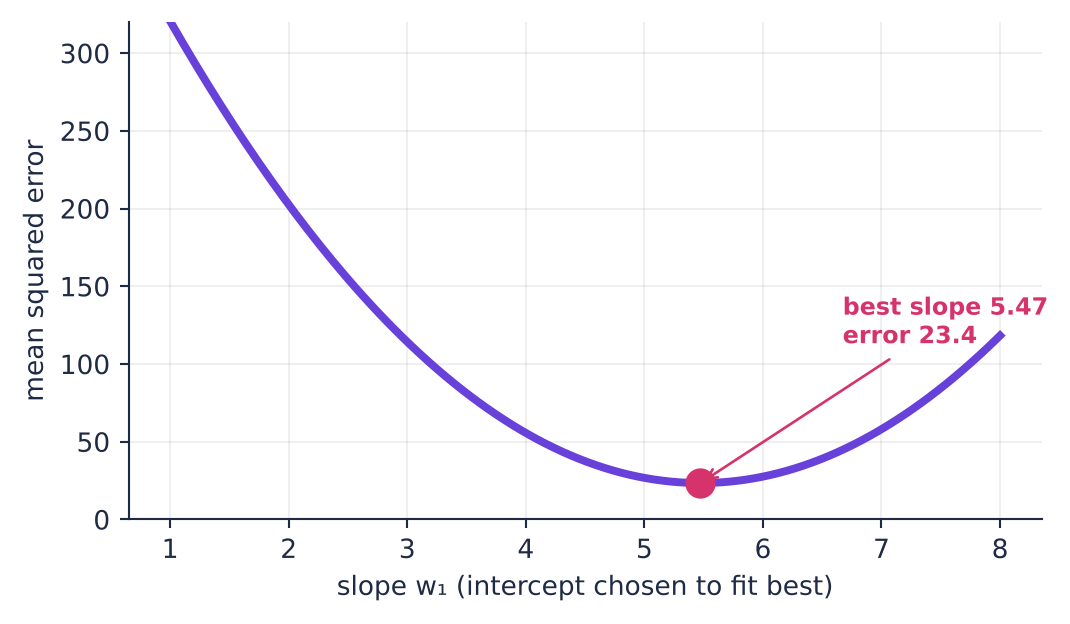
Illustration for Move the settings toward smaller error. The reading guide immediately below explains its parts and conclusion. — **Read the illustration:** The horizontal axis varies slope while the intercept is fixed at the book’s chosen value. The vertical axis is training MSE. The bottom is the best slope on this slice, not a complete picture of every parameter combination.
Source: Linear Regression · Book 8, PDF pages 8–10. Static source illustration; annotated scores belong to this example.

Move the settings toward smaller error: compare the quantities
Method	What it does
Least squares	Solve the linear fit numerically
Gradient descent	Repeat local updates
Validation	Check usefulness on unseen cases

w_new = w_old − learning_rate × loss_gradient

A gradient is a local sensitivity. Subtracting it proposes a downhill step; the learning rate scales that step.

Return to the playground and explain how its inputs connect to this relationship. Unscored reading.