Equation X-Ray · Read the structure, then explain it
Mathematics as a language
Read a prediction before adjusting it
Estimate a house price from area without confusing the estimate with its observed sale price.
ŷ = wx + b
Read the relationship before trying to solve it. This is an illustrative example, separate from the live experiment.
Choose a building block to inspect its role.
Read the operations: At x=2.5, multiply 42 × 2.5 = 105, then add 140 to get 245.
Build the expression from smaller operations
Choose a valid construction in the stated order. This exercise organizes dependencies; it does not claim every implementation must evaluate independent branches in this order.
What problem could this relationship represent?
A rate plus a baseline also describes many non-housing relationships.
Context we still need: A model relationship does not prove that changing area causes a price change in the world.
Connect the operations to code
prediction = coefficient * area + baselineRead the code as a map of operations. It is not executed here; imports, shapes and numerical safeguards depend on the actual lesson.
Explain a changed situation
Review the five-level equation-reading journey →
Your notes and reveals are temporary. This reading practice does not change lesson completion or saved assessment evidence.
From a rule of thumb to an equation
1 · Observe
Say it in words first
| Word | What it means |
|---|---|
| Weight (w) | How much the prediction moves for each extra unit of the input. Here lakh per sq m. |
| Bias or intercept (b) | The line's starting height, its value when the input is zero. It lifts or lowers the whole line. |
| Equation ŷ = w·x + b | The prediction: multiply the input by the weight, then add the bias. |
| Error | How far a prediction is from the real value. |
| MSE | Mean squared error: square each miss, then average. Big misses count extra. |
An agent might say: 'each extra square metre adds about ₹80,000, and there is a small fixed adjustment'. That sentence is already a linear regression. The equation just gives its two ingredients names.
2 · Express
The equation
Different (w, b) pairs draw different lines. To compare them we need one number that says how far a line is from the sales. The usual choice is the mean squared error (MSE): square each miss, then average.
3 · Visualize
Three candidate rules
Same eight flats as before. We try three rules and compute the mean squared error for each.
| Rule | MSE |
|---|---|
| 0.5 × area + 0 | 330.1 |
| 0.8 × area − 8 | 23.6 |
| 0.81 × area − 6.8 | 21.1 |
The first rule is badly off. The second is close. The third, the fitted line rounded to two decimals, is the best of the three. The best possible line, with unrounded numbers, has an MSE of 21.0.
- Sales
- 0.5 x area + 0 (MSE 330.1)
- 0.8 x area − 8 (MSE 23.6)
- Fitted line (MSE 21.1)
See the numbers behind this picture
| Area (sq m) | Sales | 0.5 x area + 0 (MSE 330.1) | 0.8 x area − 8 (MSE 23.6) | Fitted line (MSE 21.1) |
|---|---|---|---|---|
| 35 | – | 17.5 | 20 | 21.387 |
| 40 | 30 | – | – | – |
| 50 | 34 | – | – | – |
| 60 | 36 | – | – | – |
| 70 | 52 | – | – | – |
| 80 | 55 | – | – | – |
| 90 | 58 | – | – | – |
| 100 | 80 | – | – | – |
| 110 | 84 | – | – | – |
| 115 | – | 57.5 | 84 | 85.863 |
4 · Discover
Reading w and b
w = 0.806 lakh per sq m, which is ₹80,600 for each extra square metre. b = −6.82 lakh is the line's value at area 0, a place no real flat lives. The intercept is a bookkeeping number that makes the line sit at the right height, not a price anyone pays.
5 · Apply
Two worked examples
Example 1, a prediction. For a 75 sq m flat: 0.806 × 75 + (−6.82) = 53.63 lakh.
Example 2, changing the rule. Raise w from 0.806 to 0.9 and keep b: a 100 sq m flat moves from 73.8 to 83.2 lakh. A change of 0.094 in w moves the prediction by 0.094 × 100 = 9.4 lakh, which is why w must be chosen carefully.
6 · Where it goes wrong
Three ways it goes wrong
7 · In Python
The equation in code
Here is how to implement it, step by step. The code below does exactly these steps, and every line is editable.
- Write the rule as price = w × area + b.
- Choose a pair (w, b), for example 0.8 and −8.
- Predict every flat's price with that pair.
- Square each miss and average them to get the MSE.
- Try other pairs. The pair with the smallest MSE is the better line.
import numpy as np

area = np.array([40, 50, 60, 70, 80, 90, 100, 110], float)
price = np.array([30, 34, 36, 52, 55, 58, 80, 84], float)
w, b = np.polyfit(area, price, 1)

x = 75
print("by hand: w * x + b =", round(w, 4), "*", x, "+", round(b, 3), "=", round(w * x + b, 2))
print("each extra sq m adds", round(w * 100, 1), "thousand rupees (w =", round(w, 3), "lakh per sq m)")
print("a flat of zero area is predicted at", round(b, 2), "lakh -> the intercept is a baseline, not a real flat")
for guess_w, guess_b in [(0.5, 0), (0.8, -8), (round(w, 2), round(b, 1))]:
    err = np.mean((price - (guess_w * area + guess_b)) ** 2)
    print("rule", guess_w, "x area +", guess_b, "-> mean squared error", round(err, 1))
by hand: w * x + b = 0.806 * 75 + -6.821 = 53.63
each extra sq m adds 80.6 thousand rupees (w = 0.806 lakh per sq m)
a flat of zero area is predicted at -6.82 lakh -> the intercept is a baseline, not a real flat
rule 0.5 x area + 0 -> mean squared error 330.1
rule 0.8 x area + -8 -> mean squared error 23.6
rule 0.81 x area + -6.8 -> mean squared error 21.1Edit and run this code in your browser
Live Python
Predict by hand and score three candidate rules
Runs in your browser on your device. Nothing you type is sent anywhere, and nothing here changes your saved progress.
Press Ctrl+Enter (⌘+Enter on Mac) to run. Tab moves focus to the next control, as usual; use spaces to indent.
Want to implement it? Open the step-by-step playbook · How to choose a model
Problem and motivation
A fictional housing analyst estimates a 2,500 ft² home's price. Its known area is 2.5 thousand ft². The rule estimates ₹245 lakh; the recorded sale price is ₹246 lakh. An estimate is a calculation, not an observed fact. Prices are in ₹ lakh (1 lakh = 100,000 rupees).
Build the intuition
Start with a baseline of 140 ₹ lakh, then add 42 ₹ lakh for each thousand ft². Across 2.5 area units the contribution is 105 ₹ lakh; adding the baseline once gives 245 ₹ lakh. Area describes the home; coefficient (weight) and baseline (bias) are model settings. The recorded price is used afterward to judge the estimate, not to calculate it.
What you will learn
Explain what moves the line
- Calculate a prediction from its input, weight and bias.
- Explain the slope effect at positive, zero and negative inputs.
- Interpret bias changes and avoid causal claims.
- Calculate a residual and explain its sign.
Guided experiment
Keep this home and its recorded price fixed. Predict a coefficient change before trying it; compare two inputs to distinguish a coefficient from a baseline.
Choose a direction, including Not sure, then try the controlled change. Review is available without recording an experiment.
Predict before changing the rule
Keep area 2.5 thousand ft² and baseline 140 ₹ lakh fixed. Change only the coefficient from 42 to 46 ₹ lakh per thousand ft². What will happen to this home's estimate?
Build the evidence
0 of 4 checks complete. Experiment interaction still required.
Completion records these objectives locally; it does not award mastery. Independent mastery will require unfamiliar examples and critical-objective evidence in the later assessment.
Explore the book’s separate housing example
A useful prediction starts with a question
A buyer asks what an unlisted flat might cost. Past sales supply observed areas and recorded prices. A model supplies an estimate for a new area; it does not reveal a hidden true price.
The playground uses a separate dataset. Compare with the illustrated example ↓
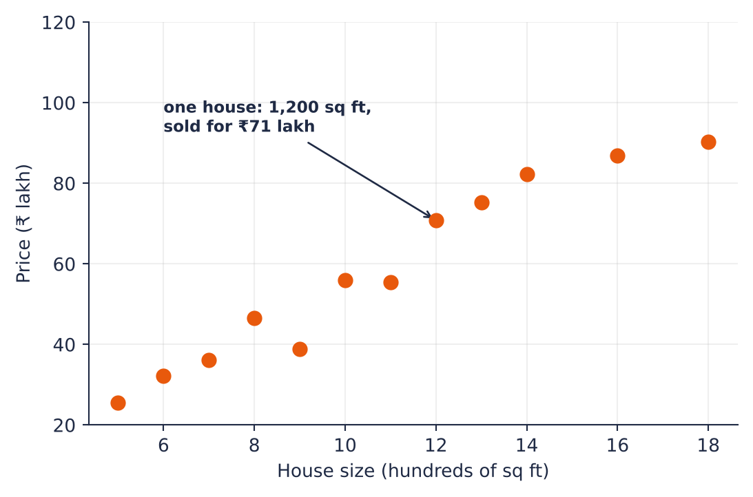
Source: Linear Regression · Book 8, PDF pages 4–5. Static source illustration; annotated scores belong to this example.
| Quantity | Role |
|---|---|
| Area | Known input |
| Recorded price | Observed target |
| Predicted price | Calculated estimate |
predicted price = intercept + slope × area
The feature is the supplied area; the target is the recorded sale price. Training chooses the slope and intercept using permitted past observations.
Return to the playground and explain how its inputs connect to this relationship. Unscored reading.